12 Types of Neural Networks Activation Functions:   Howto Choose?

What is a Neural Network Activation Function?

An Activation Function decides whether a neuron should be activated or not. This means that it will decide whether the neuron’s input to the network is important or not in the process of prediction using simpler mathematical operations. 

The role of the Activation Function is to derive output from a set of input values fed to a node (or a layer).

Depending on the nature and intensity of these input signals, the brain processes them and decides whether the neuron should be activated (“fired”) or not. 

The primary role of the Activation Function is to transform the summed weighted input from the node into an output value to be fed to the next hidden layer or as output.

Why do Neural Networks Need an Activation Function?

So we know what Activation Function is and what it does, but— 
Why do Neural Networks need it?
Well, the purpose of an activation function is to add non-linearity to the neural network.

Binary Step Function

The binary step function depends on a threshold value that decides whether a neuron should be activated or not. 

The input fed to the activation function is compared to a certain threshold; if the input is greater than it, then the neuron is activated, else it is deactivated, meaning that its output is not passed on to the next hidden layer.

Mathematically it can be represented as:

Here are some of the limitations of the binary step function:

• It cannot provide multi-value outputs—for example, it cannot be used for multi-class classification problems. 
• The gradient of the step function is zero, which causes a hindrance in the backpropagation process.

Sigmoid / Logistic Activation Function 

This function takes any real value as input and outputs values in the range of 0 to 1. 
The larger the input (more positive), the closer the output value will be to 1.0, whereas the smaller the input (more negative), the closer the output will be to 0.0, as shown below.

Sigmoid/Logistic Activation Function

Mathematically it can be represented as:

Here’s why sigmoid/logistic activation function is one of the most widely used functions:

• It is commonly used for models where we have to predict the probability as an output. Since probability of anything exists only between the range of 0 and 1, sigmoid is the right choice because of its range.
• The function is differentiable and provides a smooth gradient, i.e., preventing jumps in output values. This is represented by an S-shape of the sigmoid activation function. 
  

The limitations of sigmoid function are discussed below:

• The derivative of the function is f'(x) = sigmoid(x)*(1-sigmoid(x)). 

The derivative of the Sigmoid Activation Function

‍
As we can see from the above Figure, the gradient values are only significant for range -3 to 3, and the graph gets much flatter in other regions. 

It implies that for values greater than 3 or less than -3, the function will have very small gradients. As the gradient value approaches zero, the network ceases to learn and suffers from the Vanishing gradient problem.

• The output of the logistic function is not symmetric around zero. So the output of all the neurons will be of the same sign. This makes the training of the neural network more difficult and unstable.
  

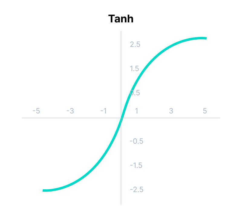
Tanh Function (Hyperbolic Tangent)

Tanh function is very similar to the sigmoid/logistic activation function, and even has the same S-shape with the difference in output range of -1 to 1. In Tanh, the larger the input (more positive), the closer the output value will be to 1.0, whereas the smaller the input (more negative), the closer the output will be to -1.0.

Tanh Function (Hyperbolic Tangent)

Mathematically it can be represented as:

Advantages of using this activation function are:

• The output of the tanh activation function is Zero centered; hence we can easily map the output values as strongly negative, neutral, or strongly positive.
• Usually used in hidden layers of a neural network as its values lie between -1 to; therefore, the mean for the hidden layer comes out to be 0 or very close to it. It helps in centering the data and makes learning for the next layer much easier.

Have a look at the gradient of the tanh activation function to understand its limitations.

Gradient of the Tanh Activation Function

As you can see— it also faces the problem of vanishing gradients similar to the sigmoid activation function. Plus the gradient of the tanh function is much steeper as compared to the sigmoid function.

💡 Note:  Although both sigmoid and tanh face vanishing gradient issue, tanh is zero centered, and the gradients are not restricted to move in a certain direction. Therefore, in practice, tanh nonlinearity is always preferred to sigmoid nonlinearity.

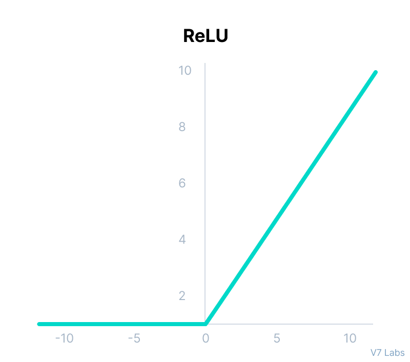
ReLU Function

ReLU stands for Rectified Linear Unit. 

Although it gives an impression of a linear function, ReLU has a derivative function and allows for backpropagation while simultaneously making it computationally efficient. 

The main catch here is that the ReLU function does not activate all the neurons at the same time. 

The neurons will only be deactivated if the output of the linear transformation is less than 0.

ReLU Activation Function

Mathematically it can be represented as:

The advantages of using ReLU as an activation function are as follows:

• Since only a certain number of neurons are activated, the ReLU function is far more computationally efficient when compared to the sigmoid and tanh functions.
• ReLU accelerates the convergence of gradient descent towards the global minimum of the loss function due to its linear, non-saturating property.
  

The limitations faced by this function are:

• The Dying ReLU problem, which I explained below.

The Dying ReLU problem

‍
The negative side of the graph makes the gradient value zero. Due to this reason, during the backpropagation process, the weights and biases for some neurons are not updated. This can create dead neurons which never get activated. 

• All the negative input values become zero immediately, which decreases the model’s ability to fit or train from the data properly. 

Leaky ReLU Function

Leaky ReLU is an improved version of ReLU function to solve the Dying ReLU problem as it has a small positive slope in the negative area.

Leaky ReLU

Mathematically it can be represented as:

The advantages of Leaky ReLU are same as that of ReLU, in addition to the fact that it does enable backpropagation, even for negative input values. 

By making this minor modification for negative input values, the gradient of the left side of the graph comes out to be a non-zero value. Therefore, we would no longer encounter dead neurons in that region. 

Here is the derivative of the Leaky ReLU function. 

The derivative of the Leaky ReLU function

The limitations that this function faces include:

• The predictions may not be consistent for negative input values. 
• The gradient for negative values is a small value that makes the learning of model parameters time-consuming.

Parametric ReLU Function

Parametric ReLU is another variant of ReLU that aims to solve the problem of gradient’s becoming zero for the left half of the axis. 

This function provides the slope of the negative part of the function as an argument a. By performing backpropagation, the most appropriate value of a is learnt.

Parametric ReLU

‍

Mathematically it can be represented as:

Where "a" is the slope parameter for negative values.

The parameterized ReLU function is used when the leaky ReLU function still fails at solving the problem of dead neurons, and the relevant information is not successfully passed to the next layer. 

This function’s limitation is that it may perform differently for different problems depending upon the value of slope parameter a.

Exponential Linear Units (ELUs) Function

Exponential Linear Unit, or ELU for short, is also a variant of ReLU that modifies the slope of the negative part of the function. 

ELU uses a log curve to define the negativ values unlike the leaky ReLU and Parametric ReLU functions with a straight line.

ELU Activation Function

Mathematically it can be represented as:

ELU is a strong alternative for f ReLU because of the following advantages:

• ELU becomes smooth slowly until its output equal to -α whereas RELU sharply smoothes.
• Avoids dead ReLU problem by introducing log curve for negative values of input. It helps the network nudge weights and biases in the right direction.
  

The limitations of the ELU function are as follow:

• It increases the computational time because of the exponential operation included
• No learning of the ‘a’ value takes place
• Exploding gradient problem

ELU Activation Function and its derivative

Mathematically it can be represented as:

‍

Softmax Function

Before exploring the ins and outs of the Softmax activation function, we should focus on its building block—the sigmoid/logistic activation function that works on calculating probability values. 

Probability

‍

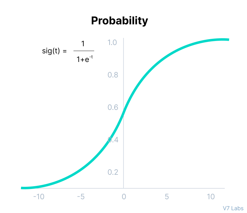
The output of the sigmoid function was in the range of 0 to 1, which can be thought of as probability. 

But—

This function faces certain problems.

Let’s suppose we have five output values of 0.8, 0.9, 0.7, 0.8, and 0.6, respectively. How can we move forward with it?

The answer is: We can’t.

The above values don’t make sense as the sum of all the classes/output probabilities should be equal to 1. 

You see, the Softmax function is described as a combination of multiple sigmoids. 

It calculates the relative probabilities. Similar to the sigmoid/logistic activation function, the SoftMax function returns the probability of each class. 

It is most commonly used as an activation function for the last layer of the neural network in the case of multi-class classification. 

Mathematically it can be represented as:

Softmax Function

Let’s go over a simple example together.

Assume that you have three classes, meaning that there would be three neurons in the output layer. Now, suppose that your output from the neurons is [1.8, 0.9, 0.68].

Applying the softmax function over these values to give a probabilistic view will result in the following outcome: [0.58, 0.23, 0.19]. 

The function returns 1 for the largest probability index while it returns 0 for the other two array indexes. Here, giving full weight to index 0 and no weight to index 1 and index 2. So the output would be the class corresponding to the 1st neuron(index 0) out of three.

You can see now how softmax activation function make things easy for multi-class classification problems.